

Keith Laker
The OLAP Extension is now available in SQL Developer 4.0
See http://www.oracle.com/technetwork/developer-tools/sql-developer/downloads/sqldev-releasenotes-v4-1925251.html for the details.
The OLAP functionality is mentioned toward the bottom of the web page.
- Manage and enable cube and dimension MV's.
- Manage data security.
- Create and edit nested measure folders (i.e. measure folders that are children of other measure folders)
- Create and edit Maintenance Scripts
- Manage multilingual support for OLAP Metadata objects
- Use the OBIEE plugin or the Data Validation plugin
- New Calculation Expression editor for calculated measures. This allows the user to nest different types to calculated measures easily. For instance a user can now create a Moving Total of a Prior Period as one calculated measure. In AWM, it would have required a user to create a Prior Period first and then create a Moving Total calculated measure which referred to the Prior Period measure. Also the new Calculation Expression editor displays hypertext helper templates when the user selects the OLAP API syntax in the editor.
- Support for OLAP DML command execution in the SQL Worksheet. Simply prefix OLAP DML commands by a '~' and then select the execute button to execute them on the SQL Worksheet. The output of the command will appear in the DBMS Output Window if it is opened, or the Script Output Window if the user has executed 'set serveroutput on' before executing the DML command.
- Improved OLAP DML Program Editor integrated within the SQL Developer framework.
- New diagnostic reports in the SQL Developer Report navigator.
- Ability to create a fact view with a measure dimension (i.e. "pivot cube"). This functionality is accessible from the SQL Developer Tools-OLAP menu option.
- Cube scripts have been renamed to Build Specifications and are now accessible within the Create/Edit Cube dialog. The Build Specifications editor there, is similar to the calculation expression editor as far as functionality.
Oracle SQL Developer Data Modeler 3.3 now available

http://www.oracle.com/technetwork/developer-tools/datamodeler/overview/index.html
Attention all data modellers - we are pleased to announce the release of SQL Developer Data Modeler 3.3. This release includes a new search, reports can be generated from search results, extended Excel import and export capabilities and more control and flexibility in generating your DDL. Here are a few links to get you started:
- For downloads see here: http://www.oracle.com/technetwork/developer-tools/datamodeler/downloads/index.html
- For information about new features see here: http://www.oracle.com/technetwork/developer-tools/datamodeler/datamodeler-33-newfeatures-1869156.html
- The release notes are available here: http://www.oracle.com/technetwork/developer-tools/datamodeler/data-modeler-releasenotes33-1869517.html
- The documentation can be found here: http://www.oracle.com/pls/topic/lookup?ctx=E29463_01&id=homepage
For data warehouse data modellers there are some very important new features around logical models, multi-dimensional models and physical models. For example:
- Support for surrogate keys during engineering to relational model which can be set on each entity.
- More flexible transformation to relational model with mixed engineering strategies based on “engineer” flag and subtypes setting for each entity in the hierarchy
- Export to “Oracle AW” now supports Oracle 11g OLAP
- Support for role playing dimensions in export to Oracle AW.
- Level descriptive attributes can be created without mapping to attribute in logical model.
- Multidimensional model can be bound directly to relational model.
- Support EDITIONING option on views, and support for invisible indexes in Oracle 11g physical model.
Lots of great features that will make life a lot easier for data warehouse teams.
Starbucks 1TB cube in production
Starbucks Coffee Company Delivers Daily, Actionable Information to Store Managers, Improves Business Insight with High Performance Data Warehouse
( http://www.oracle.com/us/corporate/customers/customersearch/starbucks-coffee-co-1-exadata-ss-1907993.html )
By delivering extreme performance combined with the architectural simplicity and sophisticated multidimensional calculation power of the in-database analytics of the Database, Starbucks use of OLAP has enabled some outstanding results. Together with the power of other Oracle Database and Exadata benefits such as Partitioning, Hybrid Columnar Compression, Storage Indexes and Flash Memory, Starbucks is able to handle the constant growth in data volumes and end-user demands with ease.
A great example of the power of the "Disk To Dashboard" capability of Oracle Business Analytics.
Webcast: Using Oracle OLAP data in multiple BI clients. Feb. 5 at 9:00 PST
Want to learn how to connect multiple BI clients such as SAP BusinessObjects Analysis, Cognos and Microsoft Excel to Oracle OLAP, quickly and easily, using the XMLA version of the MDX Provider for Oracle OLAP? Check out the Oracle webcast on February 5 at 9:00 AM PST.
You will see how it works and how customers in different industries are using this solution.
Just sign up here and join us on February 5th.
Webinar: Using XMLA with Cognos and Oracle OLAP Cubes
To attend: Sign up here.
If you use a business intelligence tool such as IBM Cognos, Microstrategy or SPA BusinessObjects Analysis that uses XMLA to connect to multidimensional data sources, check out a free webinar by Simba Technologies which offers a "sneak peak" of the Simba XMLA Provider for Oracle OLAP. The Simba XMLA Provider for Oracle OLAP is an XMLA version for the Simba MDX Provider for Oracle OLAP, the gold standard in MDX connectivity to Oracle OLAP. (The Simba MDX Provider for Oracle OLAP allows MDX based clients such as Microsoft Excel PivotTables to query Oracle OLAP cubes. The XMLA version allows clients that use XMLA rather than ODBO to connect to Oracle OLAP.)
Simba will demonstrate using IBM Cognos using the XMLA provider to query Oracle OLAP cubes. Here's a brief outline of the session.
See how:
- Familiar business intelligence applications such as IBM Cognos can connect to an Oracle OLAP cube.
- Ad-hoc querying and data analysis can be performed directly in IBM Cognos on your OLAP data.
- The most advanced application that responds to XMLA requests available enables users to interactively build reports, drill into details and slice and dice data
- Connectivity can be established without the need to install any software on the client machine.
Simply connect to the XMLA service and everything works!
Creating Oracle BI Presentation Layers from Oracle Cubes
The Oracle BI plug-in for Analytic Workspace Manager pushes metadata into the Oracle BI repository using UDML code. The result is a ready to use subject area with the Physical, Business Model and Presentation layers fully built for you. It creates hierarchies in the Business Model layer, but it does not add hierarchical columns to the Presentation layer. You can easily add hierarchical columns to the Physical layer by dragging hierarchies from the Business Model layer.
 Hierarchical column in the channel dimension.
The Oracle BI plug-in for Analytic Workspace Manager creates a Physical layer that maps to hierarchy and cube views (these views make the dimensions, hierarchies and cubes look like a star schema to SQL). In the Business Model, it assigns the SUM aggregation operator to measures selected from the cube view. This approach allows SQL to aggregate data above the cube. This is useful for queries that first filter and then aggregate and attribute break outs. For example:
- Report by Year where Quarter of Year is 3 and 4. Data at the Year level will be the aggregate of child quarters 3 and 4.
- Report by Year, Color and Size where Color and Size are attributes of Item. Oracle will SELECT year, color, size, SUM(sales) .... GROUP BY year, color, size.
In both cases, Oracle BI will get the highest aggregate level data it can from the cube and do some additional aggregation in SQL.
When cubes are imported using the Oracle BI Administration tool the Physical layer is mapped directly to the cube and dimensions, bypassing the cube and hierarchy views. The SQL created in this case selects from the OLAP_TABLE table function. Oracle BI has optimized this SQL to take advantage of some features in OLAP_TABLE, which offers better query performance with hierarchical columns in some situations.
When the cube is imported with the Oracle BI Administration tool, aggregation is set to 'External Aggregation'. This will disable the ability to create queries that require aggregation above the cube. This is good in that it prevents users creating queries that might not work as they expect in some cases, but it prevents filter before aggregate and attribute break out queries.
Also, the import method only creates the Physical layer. It does not create the Business Model and Presentation layers. You do that by dragging the Physical layer to the Business Model layer and then dragging the Business Model to the Presentation layer. That's all quick and easy, but there will be some things you will want to update in the Business Model and Presentation layers. For example, deleting some columns you don't really need and arranging columns in hierarchical order. I've posted the paper Creating an Oracle BI Presentation Layer from Oracle Cubes on OTN. This paper will walk you through the process of refining the Business Model and Presentation layers.
My recommendation is to try each method, learn about the strengths of each and choose which is best for any particular application. Since all the data comes from the same cube, there's nothing wrong with using both methods.
Introduction to Oracle OLAP Web Presentation Series
Oracle OLAP Overview: Part 1 - Architecture
Oracle OLAP Overview: Part 2 - Key Features
Oracle OLAP Overview: Part 3 - Use Cases
Creating Custom (Calculated) Members
Let's look at an example using the OLAPTRAIN schema. Suppose you want the total of the states in the northeastern United States. In OLAPTRAIN, that would include Massachusetts, Rhode Island, New York and Pennsylvania..
If you did this with SQL, it might look something like this.
g.country_long_description AS country,
p.all_products_long_descri AS all_products,
c.all_channels_long_descri AS all_channels,
SUM(f.sales)
FROM time_calendar_view t,
product_standard_view p,
geography_regional_view g,
channel_sales_channel_view c,
sales_cube_view f
WHERE t.dim_key = f.time
AND p.dim_key = f.product
AND g.dim_key = f.geography
AND c.dim_key = f.channel
AND t.level_name = 'CALENDAR_YEAR'
AND p.level_name = 'ALL_PRODUCTS'
AND c.level_name = 'ALL_CHANNELS'
AND g.level_name = 'STATE_PROVINCE'
AND g.state_province_long_desc IN ('Massachusetts','Rhode Island','New York', 'Pennsylvania')
AND t.calendar_year_long_descr = 'CY2009'
AND g.country_long_description = 'United States'
GROUP BY t.calendar_year_long_descr,
g.country_long_description,
p.all_products_long_descri,
c.all_channels_long_descri;
And the query would return as
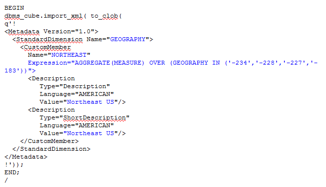
A different way to approach this is to create a custom member that is the aggregate of other members. In this case, the custom member is added to the dimension and can be used just like any other dimension member. The only real difference is that a custom member is not within a hierarchy and does not belong to a level. The advantages are that the custom member is available to all users (unless you control access, more on that later), they work with all of the cube's aggregation rules (e.g., first, last, hierarchical weighted average and so on), they work seamlessly with calculated measures and they are available in all tools (e.g., Excel PivotTables).
Custom aggregates are created using the dbms_cube.import program. Note that the dimension keys are numeric in OLAPTRAIN. (Sorry for posting this sample as an image ... blogger wasn't happy about displaying XML. To view the full example option the image in a new tab or window).
g.long_description AS geog,
p.long_description AS product,
c.long_description AS channel,
f.sales
FROM time_calendar_view t,
product_standard_view p,
geography_regional_view g,
channel_sales_channel_view c,
sales_cube_view f
WHERE t.dim_key = f.time
AND p.dim_key = f.product
AND g.dim_key = f.geography
AND c.dim_key = f.channel
AND t.level_name = 'CALENDAR_YEAR'
AND p.level_name = 'ALL_PRODUCTS'
AND c.level_name = 'ALL_CHANNELS'
AND g.long_description = 'Northeast US'
AND t.calendar_year_long_descr = 'CY2009';
Fine Tuning Incremental Updates using LOAD PRUNE
With a little bit of effort, you can improve update times by writing your own cube processing script. You can also use MV log tables to automatically captured changes made to the fact table and use them as the data sources to cube updates.
AWM defines and makes the LOAD_AND_AGGREGATE script the default script of the cube. If you don’t specify a different script, LOAD_AND_AGGREGATE is automatically used as shown in the following example (note that the script references the OLAPTRAIN.SALES_CUBE but does not including the USING clause).
BEGIN
DBMS_CUBE.BUILD('OLAPTRAIN.SALES_CUBE','C',false,4,true,true,false);
END;
/
This script will run the LOAD PARALLEL and SOLVE PARALLEL commands. What this means is that for each partition, the database will LOAD data from the fact table/view and then SOLVE (aggregate) data. If you have specified a value for parallel that is greater than 1, partitions will be processed in parallel (in the example above, 4 processes). AWM also provides the ability to set the refresh method (C, or complete, in the above example).
LOAD_AND_AGGREGATE is a good choice for a full build, but it might not be the best choice for an incremental update. If you are simply updating the cube with changes within a few recent partitions (e.g., yesterday or this month), the LOAD PRUNE command is probably better than LOAD PARALLEL.
LOAD PRUNE will first query the fact table or view to first determine which partition will have new data using a SELECT DISTINCT. It will then only generate LOAD commands for those partitions that will have records loaded into them.
Let’s run through an update scenario. Make the following assumptions:
* The time dimension has months for 2008 through 2012 and the cube is partitioned by month. The cube will have 60 partitions.
* You have loaded data into the cube for January 2008 through March 2012.
* It’s now time to load data for April 2012. This data has been inserted into the fact table.
* You have mapped the cube to a view. For the April 2012 update, you have added a filter to the view so that it returns data only for April.
If you use the LOAD_AND_AGGREGATE script and choose the FAST SOLVE refresh method, the database will really to the following:
BEGIN
DBMS_CUBE.BUILD('OLAPTRAIN.SALES_CUBE USING (LOAD PARALLEL, SOLVE PARALLEL)','S',false,4,true,true,false);
END;
/
With LOAD PARALLEL, the database will process the LOAD command for each partition (all 60). Since it’s selecting from a view that’s filtered out all but April 2012, 59 partitions will have no new or changed data. Although it doesn’t take a long time to load 0 rows and figure out that a SOLVE is not required, it still adds up if there are a lot of partitions.
With LOAD PRUNE, the database will determine that a LOAD is only required for April 2012. The LOAD step is skipped for all other partitions. While you will still see the SOLVE for all partitions, it doesn’t really do any work because no rows were loaded into the partition. An example using LOAD PRUNE follows.
BEGIN
DBMS_CUBE.BUILD('OLAPTRAIN.SALES_CUBE USING (LOAD PRUNE, SOLVE PARALLEL)','S',false,2,true,true,false);
END;
/
If you would like a script that walked through a complete example using the OLAPTRAIN schema, including the use of an MV log table to automatically capture changes to the fact table, send me an email william.endress@oracle.com with a link to this posting.
Excel and OLAP: ODBC vs. MDX
The answer really boils down to leveraging meta data and automatic query generation.
With ODBC, it's up to the Excel user to write a SQL query to fetch data from the cube. Data can be returned in tabular format or a pivot table. When the data is viewed in a pivot table Excel will aggregate data, sometimes with unexpected results. For example Excel might choose to aggregate a measure such as Sales with COUNT or might try to SUM a measure such as Sales YTD Percent Change. Neither make any sense. It's up to the user to get it right.
With the MDX Provider, Excel understands what all the columns mean. It understands dimensions, hierarchies and levels. It's understand the difference between a key and a label. It knows what a measure is. It allows the server to calculate the data. Query generation is automatic. Business users just choose hierarchies and measures and the MDX Provider does the rest.
Here's a list of some of the advantages of using the MDX Provider for Oracle OLAP as compared to using ODBC and writing your own SQL.

Oracle OLAP Exadata Performance Demonstration
http://www.oracle.com/technetwork/database/options/olap/olap-exadata-x2-2-performance-1429042.pdf
The Executive Overview section of this paper provides an introduction:
This paper describes a performance demonstration of the OLAP Option to the Oracle Database running on an X2-2 Exadata Database Machine half rack. It shows how Oracle OLAP cubes can be used to enhance the performance and analytic content of the data warehouse and business intelligence solutions, supporting a demanding user community with ultrafast query and rich analytic content.
The demonstration represents users of a business intelligence application using SQL to query an Oracle OLAP cube that has been enhanced with a variety of analytic measures. The cube contains data loaded from a fact table with more than 1 billion rows.
Utilizing Exadata features such as Smart Flash Cache, Oracle Database supported a community of 50 concurrent users querying the cube with queries that are typical of those executed from a business intelligence tool such as Oracle Business Intelligence Enterprise Edition.
With each user querying the database non-stop (without waits between queries) with median query times ranged from .03 to .58 seconds, average query times ranged from .26 to 2.32 seconds, and 95 percent of queries returned in 1.5 to 5.5 seconds, depending on the type of query.
Query performance can be attributed to highly optimized data types and Exadata Smart Flash Cache. Cubes are designed for fast access to random data points, using features such as array-based storage, cost-based aggregation, and joined cube scans. Exadata Smart Flash Cache contributes significantly to cube query performance, virtually eliminating IO wait for the high volume, random IO typically seen with cube queries.
Script for Time Dimension Table
One of the more common requests I get is a script for creating time dimension tables for Oracle OLAP. The following script will create a time dimension table for a standard calendar. It starts by creating a table with dimension members and labels. The second part of the script fills in end date and time span attributes. The section that creates end date and time span can be easily adapted for completing other calendars (e.g., fiscal) where the members have already been filled in.
-- Create time dimension table for a standard calendar year (day, month,
-- quarter, half year and year).
--
-- Drop table.
--
--DROP TABLE time_calendar_dim;
--
-- Create time dimension table for calendar year.
--
-- First day if the next day after TO_DATE('31/12/2010','DD/MM/YYYY').
-- Number of days is set in CONNECT BY level <= 365.
--
-- Values for end date and time span attributes are place holders. They need
-- to be filled in correctly later in this script.
--
CREATE TABLE time_calendar_dim AS
WITH base_calendar AS
(SELECT CurrDate AS Day_ID,
1 AS Day_Time_Span,
CurrDate AS Day_End_Date,
TO_CHAR(CurrDate,'Day') AS Week_Day_Full,
TO_CHAR(CurrDate,'DY') AS Week_Day_Short,
TO_NUMBER(TRIM(leading '0'
FROM TO_CHAR(CurrDate,'D'))) AS Day_Num_of_Week,
TO_NUMBER(TRIM(leading '0'
FROM TO_CHAR(CurrDate,'DD'))) AS Day_Num_of_Month,
TO_NUMBER(TRIM(leading '0'
FROM TO_CHAR(CurrDate,'DDD'))) AS Day_Num_of_Year,
UPPER(TO_CHAR(CurrDate,'Mon')
|| '-'
|| TO_CHAR(CurrDate,'YYYY')) AS Month_ID,
TO_CHAR(CurrDate,'Mon')
|| ' '
|| TO_CHAR(CurrDate,'YYYY') AS Month_Short_Desc,
RTRIM(TO_CHAR(CurrDate,'Month'))
|| ' '
|| TO_CHAR(CurrDate,'YYYY') AS Month_Long_Desc,
TO_CHAR(CurrDate,'Mon') AS Month_Short,
TO_CHAR(CurrDate,'Month') AS Month_Long,
TO_NUMBER(TRIM(leading '0'
FROM TO_CHAR(CurrDate,'MM'))) AS Month_Num_of_Year,
'Q'
|| UPPER(TO_CHAR(CurrDate,'Q')
|| '-'
|| TO_CHAR(CurrDate,'YYYY')) AS Quarter_ID,
TO_NUMBER(TO_CHAR(CurrDate,'Q')) AS Quarter_Num_of_Year,
CASE
WHEN TO_NUMBER(TO_CHAR(CurrDate,'Q')) <= 2
THEN 1
ELSE 2
END AS half_num_of_year,
CASE
WHEN TO_NUMBER(TO_CHAR(CurrDate,'Q')) <= 2
THEN 'H'
|| 1
|| '-'
|| TO_CHAR(CurrDate,'YYYY')
ELSE 'H'
|| 2
|| '-'
|| TO_CHAR(CurrDate,'YYYY')
END AS half_of_year_id,
TO_CHAR(CurrDate,'YYYY') AS Year_ID
FROM
(SELECT level n,
-- Calendar starts at the day after this date.
TO_DATE('31/12/2010','DD/MM/YYYY') + NUMTODSINTERVAL(level,'DAY') CurrDate
FROM dual
-- Change for the number of days to be added to the table.
CONNECT BY level <= 365
)
)
SELECT day_id,
day_time_span,
day_end_date,
week_day_full,
week_day_short,
day_num_of_week,
day_num_of_month,
day_num_of_year,
month_id,
COUNT(*) OVER (PARTITION BY month_id) AS Month_Time_Span,
MAX(day_id) OVER (PARTITION BY month_id) AS Month_End_Date,
month_short_desc,
month_long_desc,
month_short,
month_long,
month_num_of_year,
quarter_id,
COUNT(*) OVER (PARTITION BY quarter_id) AS Quarter_Time_Span,
MAX(day_id) OVER (PARTITION BY quarter_id) AS Quarter_End_Date,
quarter_num_of_year,
half_num_of_year,
half_of_year_id,
COUNT(*) OVER (PARTITION BY half_of_year_id) AS Half_Year_Time_Span,
MAX(day_id) OVER (PARTITION BY half_of_year_id) AS Half_Year_End_Date,
year_id,
COUNT(*) OVER (PARTITION BY year_id) AS Year_Time_Span,
MAX(day_id) OVER (PARTITION BY year_id) AS Year_End_Date
FROM base_calendar
ORDER BY day_id;
);
--
COMMIT;
Simba previews Cognos8 Analysis Studio accessing Oracle Database OLAP Option cubes
- Oracle BIEE 10g and 11g (see http://oracleolap.blogspot.com/2010/07/first-look-at-obiee-11g-with-oracle.html ) and
- Oracle BI Discoverer Plus OLAP (see http://oracleolap.blogspot.com/2010/08/discoverer-olap-is-certified-with-olap.html ),
&amp;amp;amp;amp;amp;amp;amp;amp;amp;amp;amp;amp;amp;amp;amp;amp;amp;amp;amp;amp;amp;lt;/param&amp;amp;amp;amp;amp;amp;amp;amp;amp;amp;amp;amp;amp;amp;amp;amp;amp;amp;amp;amp;amp;gt;&amp;amp;amp;amp;amp;amp;amp;amp;amp;amp;amp;amp;amp;amp;amp;amp;amp;amp;amp;amp;amp;lt;param name="allowFullScreen" value="true" frameborder="0"&amp;amp;amp;amp;amp;amp;amp;amp;amp;amp;amp;amp;amp;amp;amp;amp;amp;amp;amp;amp;amp;gt;
Simba previews Oracle OLAP MDX Provider connectivity to SAP BusinessObjects Voyager
This will be a great capability for users of both Oracle OLAP and BusinessObjects and will futher extend the reach of Oracle database embedded OLAP cubes.
You can get more details on the Simba website
Microsoft Certifies Simba’s MDX Provider for Oracle OLAP as “Compatible with Windows 7”
Cell level write-back via PL/SQL
Since the first OLAP Option release in 9i it has always been possible to write-back to cubes via the Java OLAP API and OLAP DML. But in recent releases, a new PL/SQL package based API has been developed. My thanks go to the ever-excellent David Greenfield of the Oracle OLAP product development group for bringing this to my attention.
At the most simple level, it is possible to write to a qualified cell:
dbms_cube.build(
'PRICE_COST_CUBE USING (
SET PRICE_COST_CUBE.PRICE["TIME" = ''24'', PRODUCT = ''26''] = 711.61, SOLVE)')
In the example above, a cube solve is executed after the cell write. The objects are referenced by their logical (ie. AWM) names.
This approach is very flexible. For example you can qualify only some dimensions, in this case the assignment is for all products:
dbms_cube.build(
'PRICE_COST_CUBE USING (
SET PRICE_COST_CUBE.PRICE["TIME" = ''24''] = 711.61, SOLVE)')
You can also skip the aggregation:
dbms_cube.build(
'PRICE_COST_CUBE USING (
SET PRICE_COST_CUBE.PRICE["TIME" = ''24'', PRODUCT = ''26''] = 711.61)')
or run multiple cell updates in one call:
dbms_cube.build(
'PRICE_COST_CUBE USING (
SET PRICE_COST_CUBE.PRICE["TIME" = ''24'', PRODUCT = ''26''] = 711.61,
SET PRICE_COST_CUBE.PRICE["TIME" = ''27'', PRODUCT = ''27''] = 86.82,
SOLVE)');
You can also copy from one measure to another.
dbms_cube.build('UNITS_CUBE USING (SET LOCAL_CUBE.UNITS = UNITS_CUBE.UNITS'));
This will copy everything from the UNITS measure in UNITS_CUBE to the UNITS measure in the LOCAL_CUBE. You can put fairly arbitrary expressions on the right hand side and the code will attempt to loop the appropriate composite. You can also control status.
For more details, take a look at the PL/SQL reference documentation
Incremental Refresh of Oracle Cubes
- The cube will load all data from the source table.
- You can limit the data loaded into the cube by a) presenting new/changed data only via a staging table or filtered view or b) making the cube refreshable using the materialized view refresh system and using a materialized view log table.
- The cube will understand if data has been loaded into a partition. If data has not been loaded into a partition, it will not be processed (aggregated).
- If a partition has had data loaded into it, it will processed (aggregated).
- The cube will understand if a loaded value is new, changed or existing and unchanged. Only new or changed values are processed (the cube attempts to aggregate only new and changed cells and their ancestors).
- Changing parentage of a member in a non-partitioned dimension will trigger a full solve of the cube (across all partitions).
- If a member is added to a non-partitioned dimension, the cube will attempt an incremental aggregation of that dimension (that is, the new member and ancestors only).
Here are two scenarios that illustrate how this works.
1) How to trigger a lot of processing in the cube during a refresh:
- Load from the full fact table rather than a staging table, filtered view or MV log table. The full table will be loaded into the cube.
- Load data into many partitions. Each partition will need to be processed. For example, load data for the last 36 months when the cube is partitioned by time.
- Load data into large partitions. For example, partition by year or quarter rather than quarter or month. Smaller partitions will process more quickly.
- Make frequent hierarchy (parentage) changes in dimensions. For example, realign customers with new regions or reorganize the product dimension during the daily cube refresh. This will trigger a full cube refresh.
2) How to efficiently manage a daily cube refresh:
- Load from staging tables, filtered views or MV log tables where the tables/views contain only new or updated fact data. This will reduce the load step of the build. This becomes more important the larger the fact table is.
- Use as fine grained partitioning strategy as possible. This will result in smaller partitions, which process more efficiently (full or incremental refresh) and offer more opportunity for parallel processing. Also, it is likely that fewer partitions will be processed.
There can be a trade off with query performance. Typically, query performance is better when partitions are at a higher level (e.g., quarter rather than week) because there may be fewer partitions to access and less dynamic aggregation might be required. That said, the gain in refresh performance is typically much greater than the loss in query performance. Building a cube twice as fast is often more important than a small slowdown in query performance.
- Only add new data into the partitioned dimension. For example if the cube is partitioned by time, add data only for new time periods. Only the partitions with those time periods will be refreshed.
Clearly, there are many cases where data must be added to the non-partitioned dimensions. For example, new customers might be added daily. This is ok because a) new members are processed incrementally and b) new customers will likely affect only more recent partitions.
Schedule hierarchy realignments (e.g., changing parentage in product, geography and account type dimensions) weekly instead of daily. This will limit the number of times a full refresh is required. It might also allow you to scheduled the full refresh for a time where the availability of system resources is high and/or the query load is low.
The above scenarios help you understand how to most efficiently refresh a single cube. Also consider business requirements and how model the overall solution Two scenarios follow.
1) Data is available at the day, item and store levels in the fact table. The business requirements are such that all data must be available for query, but in practice most queries (e.g., 95% or more) are at the week, item and store levels.
Consider a solution where data is loaded in the cube at the week, item and city levels and more detailed data (day, item and store levels) are made available by drilling through to the table. This is very easy to do in a product such as Oracle Business Intelligence (OBIEE) or any other tool that has federated query capabilities and will be transparent to the business user.
In this case, the cube is simply smaller and will process more quickly. The compromise is that calculations defined in the cube are only available at the week, item and city levels. This is often a reasonable trade off for faster processing (and perhaps more frequent updates).
2) Data is available at the day, item and store levels in the fact table. The business requirements are such that all data must be available for query, but in practice:
- Longer term trending (e.g., year over year) is done at the week level or higher.
- Analysis of daily data (e.g., same day, week or month ago) is only done for the most recent 90 days.
In this scenario, consider a two cube solution:
- Cube A contains data at the week, item and store levels for all history (e.g., the past 36 months). This might be partitioned at the week level and aggregated to the month, quarter and year levels. Depending on reporting requirements, it might only be refreshed at the end of the week when the full week of data is available.
- Cube B contains data only at the day level for the most recent 90 days. It is not aggregated to the week, month, quarter and year levels (aggregates are serviced by Cube A). This cube is used for the daily sales analysis. This might be partitioned at the day level so that a) any full build of the cube can be highly parallelized and b) the daily update processes only a single and relatively small partition.
Using a tool such as Oracle Business Intelligence, which has federated query capabilities, a single business model can be created that accesses data from both cubes and the table transparently to the business user. When ever the user is querying at the week level or above, data OBIEE queries Cube A. If data is queried at the day level within the most recent 90 days, OBIEE queries Cube B. If data at the day level that is older than 90 days is access, OBIEE queries the table. Again, this can all be transparent to the user in a tool such as Oracle Business Intelligence.
Simba Technologies and Vlamis Software Solutions hosting special reception at OpenWorld 2010


Special OpenWorld 2010 Cocktail Reception
Simba product managers will also be available at the Oracle OLAP pod in Moscone West to answer questions you might have about Excel Pivot Tables and the MDX Provider for Oracle OLAP.
Discoverer OLAP is certified with OLAP 11g
If you are interested, you can download it from OTN under Portal, Forms, Reports and Discoverer (11.1.1.3.0)
An updated version of the BI Spreadsheet add-in has been released too and can also be downloaded from OTN